Finding Roots

Laboratory work 5.2

Mathematical analysis problems, linear algebra problems, solving optimization problems, solving differential equations, processing of experimental data with the help of application package MathCAD.

The aim of the work:

- to get acquainted with methods of the equations solving,

- to perform calculations of the equations systems,

- to study the graphical method of the equations solving.

It is known that many equations and systems of equations have no analytical solutions. First of all it is referred to most of transcendental equations. It is not possible to create the formula to solve any higher degree algebraic equation. However, these equations can be solved numerically with a given accuracy (not more than with specified system variable TOL).

This section describes how to solve equations ranging from a single equation in one unknown to large systems with multiple unknowns.

Finding Roots

root(f (z), z) - Returns the value of z which the expression f (z) is equal to 0. The arguments are a real- or complex-valued expression f (z) and a real or complex scalar, z. Must be preceded in the worksheet by a guess value for z. Returns a scalar. The root function solves a single equation in a single unknown. This function takes an arbitrary expression or function and one of the variables from the expression. root can also take a range in which the solution lies. It then varies that variable until the expression is equal to zero and lies in the specified range. Once this is done, the function returns the value that makes the expression equal zero and lies in the specified range.

root(f (z), z, a, b) - Returns the value of z lying between a and b at which the expression f (z) is equal to 0. The arguments to this function are a real-valued expression f (z), a real scalar, z, and real endpoints a<b. No guess value for z is required. Returns a scalar.

An example, of the root usage.

We find the solution to an equation with a single variable by rewriting the equation in the form f(x) = 0, and then using a root solver. The root-finding algorithm is known as the secant method. This method requires you to make an initial guess at the root. The algorithm then iterates from your guess until a true root is found. A warning is given if no root is found.

Let’s try to find the solution to the equation

x³ = e^x

First, we rewrite the equation in the form, f(x) = 0.

x³ - e^x or f(x) = x³ - e^x

Let’s examine f(x) and determine the real (i.e., not complex) roots, which are the values of x that satisfy the equation

f(x) = 0 = x³ - e^x

Because this is a cubic equation, we can anticipate that there might be multiple roots (i.e., more than one answer). However, it is not immediately clear how many real roots there are, since some of the roots may be imaginary. In any event, the root-finding algorithm will determine one root each time the algorithm is executed.

How can we ensure that distinctly different roots will be found each time? Generally, before beginning root finding we should get some idea of what the function “looks like”.

With MathCAD it is easy to do this by plotting the function. Looking at the plot, we can make reasonable guesses (estimates) for the value of the root we are trying to find.

OK. Now it’s time for you to get typing! Begin by defining the function f(x) = x³ - e^x and then plotting f(x) vs. x over the range -10<=x<=10. Use the previous lessons as a guide for how to do this quickly and easily, without separately defining x.

To observe where the function crosses the axes, f = 0, it is useful to select the “Crossed” option under “Axes Style”.

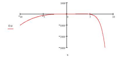
Looking at your graph, it seems that the function crosses from below the f = 0 axis into the positive region, and subsequently crosses back again into negative f region. This suggests the function has at least 2 real roots. You can find them using the ‘root’ function as follows. First, define a guess value of a root (say x = -5), and then use the root function.

x:=5

a:root(x3 - ex, x) or alternatively a:root(f(x), x)

a=

The result should be a = 1.857. Try different initial guesses. You should be able to find the second root at x = 4.536.

polyroots(v) - Returns the roots of an n th degree polynomial whose coefficients are in v, a vector of length n+1. Returns a vector of length n.

To find the roots of a polynomial or an expression having the form: you can use polyroots rather than root. polyroots does not require a guess value, and polyroots returns all roots at once, whether real or complex. Figure 1 shows examples.

Figure 1: Finding roots with root and polyroots.

By default, polyroots uses a LaGuerre method of finding roots. If you want to use the companion matrix method instead, click on the polyroots function with the right mouse button and choose Companion Matrix from the pop-up menu.

To create vector with polynomial coefficient you have to:

- put you cursor to the polynomial variable;

- choose SYMBOLS→POLINOMIAL COEFFICIENTS;

- choose EDIT→CUT;

- type v:= and choose EDIT→PASTE.

Дата добавления: 2015-10-26