Worked Example 2

Figure 4 shows a simulated material microstructure, where the black lines represent grain boundaries and the green regions represent second phase precipitates or colonies.

The analysis proceeds as follows, using the procedures shown in Figure 5 and Table 2.

1) Following the point counting method, draw a grid on the image. The lines of this grid should be spaced sufficiently that no feature is measured twice, in order to respect the random sampling criterion for us to be able to statistically analyse our results. The points where the lines cross on this grid are examined and assigned a value of 1 if they are in the second phase, 0 if they are in the matrix and 0.5 if they are on the borderline, see Figure 5a and Table 2, column 2.

2) Considering the lines on the grid, the number of interphase boundaries (boundaries between the two phases), N_{L (Inter)}, is counted, as shown in Figure 5b (for clarity, only the horizontal lines of the grid and the relevant points are shown) and Table 2, column 4.

3) The number of grain boundaries in the matrix phase (the primary phase), N_{L (GB)}, is now counted, Figure 5c and Table 2, column 6.

4) The point fraction for each line is then determined, and from these values the overall point fraction (equal to the volume fraction) for the image is found, Table 2.

5) We now use the fact that the fraction of the test lines occupied by each phase is given by the point fraction (i.e. the fact that ) to work out the linear intercept length of each phase:

a. Each second phase region has two interphase boundaries, and so the number of regions is half the number of boundaries. For lines of length L, the linear intercept length of the second phase region (the distance between two interphase boundaries) for each line, L_{L(Inter) i}, is given by:

(6)

This is calculated in Table 2, column 5. Lines where no second phase regions were measured give zero and are ignored.

b. In a similar way, the linear intercept length of the grains of the matrix phase is given by:

(7)

Here we count both the grain boundaries and the interphase boundaries, and we use the volume fraction of the matrix phase.

c. From these values for each line, the overall mean intercept lengths and errors in the measurement can be determined, as before.

d. In the case that there were also grains in the second phase regions, it would be necessary to make a further measurement of the number of intercepts with those grain boundaries, and use a formula like Eqn. (7) counting both these grain boundaries and the interphase boundaries. Should the microstructure also be anisotropic, it may be necessary to perform this analysis along multiple directions to characterise the anisotropy.

Figure 4 – An artificial 2 phase microstructure, the black lines representing grain boundaries and the green regions representing the second phase.

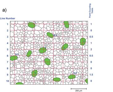
Figure 5 – The linear intercept method for grain or colony size determination in a two phase microstructure.

Table 2 – The calculation of grain size and second phase region size using the linear intercept method

Line Number, i	No. of Points in Minor Phase	Point Fraction, PP i	No. of Interphase Boundaries, NL (Inter)	Linear Intercept Length, L(Inter)i (µm)	No. of Matrix Grain Boundaries, NL (GB)	Linear Intercept Length, L(GB)i (µm)
		0.125		40.6		34.0
		0.000		-		27.8
	0.5	0.063		81.3		30.6
		0.125		81.3		27.8
		0.250		40.6		29.6
	0.5	0.063		40.6		27.0
		0.000		81.3		31.7
		0.000		-		29.6
	1.5	0.188		81.3		27.0
		0.000		54.2		30.1
		= 0.081		= 62.6 µm		= 29.5 µm

Дата добавления: 2015-10-26