Worked Example – Part 1

Figure 1 shows a simulated material microstructure, with the black circles representing second phase particles.

Figure 1 – A simulated 2 phase microstructure.

The analysis proceeds as follows, using the procedures shown in Figure 2, and in Table 1.

1) Identify an appropriate grid size for the image (with spacing large enough that no feature is sampled more than once), and draw this grid randomly on the image, Figure 2a.

2) Taking either the vertical or horizontal lines, go along the line assessing in which phases the intersections of the grid are located, and assign them the values 1 for the second phase, 0 for the primary phase, and 0.5 for the interphase boundary. Total the count for the line (Figure 2b).

3) Repeat for all of the lines (Figure 2c). The reason for treating each line like this is that we will later use the results from each line as one “measurement” of the volume fraction, which allows us to perform statistical analysis on the result.

4) For each line, i, divide this total by the total number of points per line to get the point fraction, P_{P i} (Table 1, column 3).

5) These point fractions are summed, and divided by the total number of lines to get the mean point fraction (Table 1, column 3).

6) The difference of the point fraction of each line P_{P i} from the mean point fraction is calculated and squared (Table 1, column 4).

7) This data is then used to calculate the standard deviation of the measurements using the equation given in the Statistics lecture (Table 1, column 4).

8) From the standard deviation, the standard error can be calculated using:

where n is our number of lines.

9) From the standard error, the 95% confidence limit can be calculated using the relevant t-value (e.g. from the table given in the Statistics lecture) and the result of the measurement expressed according to:

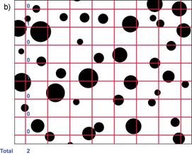
Figure 2 – The method of analysis used for point counting.

Line Number, i	No. Points in Minor Phase	Point Fraction, PP i	Difference from sample mean
		0.250	0.0002
	2.5	0.313	0.0062
		0.000	0.0550
		0.250	0.0002
		0.125	0.0120
		0.250	0.0002
	2.5	0.313	0.0062
		0.375	0.0197
		ΣPP i = 1.876	= 0.0142
		ΣPP i / 8 = 0.2345	s = 0.1193

Table 1 – The calculation of volume fraction by point counting

In this case the actual volume fraction of the second phase in the image is 0.18, so our result calculated above is not very accurate. This is reflected in the large value of the standard deviation. Using the equation for standard error, this can be calculated to be S(P_P) = 0.0422, which, as t_{(95, n-1)} is 2.365 for n=8, gives us a result that we can express with 95% confidence limits as V_V = 0.235 ± 0.100.

The true value evidently does lie inside these bounds, but the measurement has not given us a much better idea than we could have obtained from visual estimation of the volume fraction. The reason for this is linked to the small number of lines we looked at, and the small number of test points per line. Later on we will look at how this could have been predicted, and how the number of measurements required to get a certain value of the 95% confidence limit can be calculated.

Дата добавления: 2015-10-26