Working Poor More Pinched as Rich Cut Back

Understimulated

A stimulus package would send more than $100 billion to American taxpayers before the end of 2008. The theory behind the rebates is that American taxpayers will take the cash and spend it—thus providing a jolt of stimulus to the economy. But will they? In 2001, Washington sought to jolt the economy back into life with tax rebates. In all, 90 million households received some $38 billion in cash. Months later, economists discovered that households spent 20 to 40 percent of their rebates during the first three months and about another third during the following three months. People with low incomes spent more.

Source: Newsweek, February 7, 2008

17. Will $100 billion of tax rebates to American consumers increase aggregate expenditure by more than, less than, or exactly $100 billion? Explain.

The $100 billion of tax rebates increase aggregate expenditure by more than $100 billion because the spending from the $100 billion increase in disposable income has a multiplied effect on the aggregate expenditure. Part of the $100 billion increase in disposable income is spent, leading the recipients’ incomes to increase. In turn, part of this increase in income is spent, thereby further increasing aggregate expenditure.

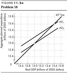
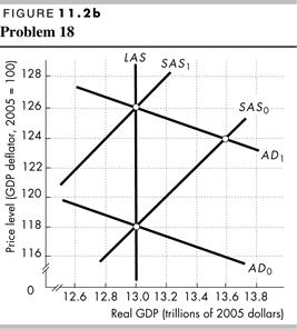
18. Explain and draw a graph to illustrate how this fiscal stimulus will influence aggregate expenditure and aggregate demand in both the short run and the long run.

Presuming the economy starts at its long-run equilibrium, Figure 11.2 shows the short-run and long-run effects on aggregate expenditure (Figure 11.2a) and on aggregate demand (Figure 11.2b). In the short run the rebate checks increase aggregate expenditure and aggregate demand. The aggregate expenditure curve shifts upward from AE ₀ to AE ₁ and the aggregate demand curve shifts rightward from AD ₀ to AD ₁. (The initial upward shift in the aggregate expenditure curve is larger but the increase in the price level moderated the initial increase in aggregate expenditure.) In the long run, however, short-run aggregate supply decreases and the short-run aggregate supply curve shifts from SAS ₀ to SAS ₁. While the higher price level does not shift the aggregate demand curve, it does shift the aggregate expenditure downward from AE ₁ back to AE ₀.

Use the following news clip to work Problems 19 to 21.

Working Poor More Pinched as Rich Cut Back

Cutbacks by the wealthy have a ripple effect across all consumer spending, said Michael P. Niemira, chief economist at the International Council of Shopping Centers. The top 20 percent of households spend about $94,000 annually, almost five times what the bottom 20 percent spent and more than what the bottom sixty percent combined spend. Then there’s also the multiplier effect: When shoppers splurge on $1,000 dinners and $300 limousine rides, that means fatter tips for the waiter and the driver. Sales clerks at upscale stores, who typically earn sales commissions, also depend on spending sprees of mink coats and jewelry. But the trickling down is starting to dry up, threatening to hurt a broad base of low-paid workers.

Source: MSNBC, January 28, 2008

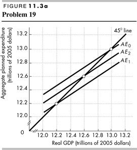
19. Explain and draw a graph to illustrate the process by which “cutbacks by the wealthy have a ripple effect.”

If the wealthy cut back on their consumption expenditure, then aggregate planned expenditure decreases. The decrease in aggregate expenditure means that aggregate demand decreases. Figure 11.3a shows the decrease in aggregate expenditure as the downward shift in the aggregate planned expenditure curve from

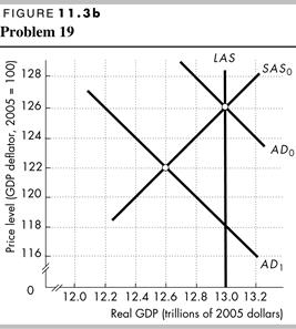
AE ₀ to AE ₁. Figure 11.3b shows the decrease in aggregate demand as the shift in the aggregate demand curve from AD ₀ to AD ₁. Figure 11.3b shows that the price level falls, from 126 to 122 in the figure. The fall in the price level increases aggregate expenditure so that the aggregate expenditure curve shifts upward from AE ₁ to AE ₂. Real GDP decreases, from $13.0 trillion to $12.6 trillion in the figures.

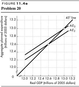
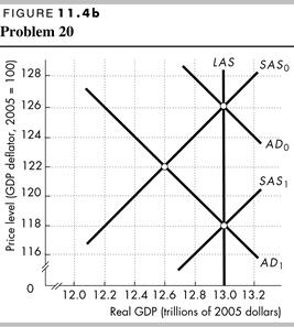
20. Explain and draw a graph to illustrate how real GDP will be driven back to potential GDP in the long run.

In the short run real GDP decreases so it is less than potential GDP, and the unemployment rate exceeds the natural unemployment rate. This higher-than-normal unemployment rate leads to a fall in the money wage rate. The fall in the money wage rate increases short-run aggregate supply, which raises real GDP and further lowers the price level. As the price level falls, aggregate expenditure increases. Eventually real GDP returns to potential GDP, at which time the price level stops falling. Figure 11.4a and 11.4b (above) show these changes. In Figure 11.4b the short-run aggregate supply curve shifts rightward from SAS ₀ to SAS ₁. In the long run the price level falls to 118. In Figure 11.4a the lower price level increases aggregate expenditure so that the aggregate expenditure curve shifts upward from AE ₂ back to AE ₀.

21. Why is the multiplier only a short-run influence on real GDP?

The multiplier has only a short-run influence on real GDP because in the long run the money wage rate changes. The change in the money wage rate affects short-run aggregate supply and lowers the price level. The fall in the price level restores aggregate planned expenditure back to its initial level and moves the economy back to its long-run equilibrium. The long-run change in aggregate expenditure offsets the initial multiplier effect on real GDP.

22. In the Canadian economy, autonomous consumption expenditure is $50 billion, investment is $200 billion, and government expenditure is $250 billion. The marginal propensity to consume is 0.7 and net taxes are $250 billion. Exports are $500 billion and imports are $450 billion. Assume that net taxes and imports are autonomous and the price level is fixed.

a. What is the consumption function?

The consumption function is the relationship between consumption expenditure and disposable income, other things remaining the same. In this case the consumption function is C = 50 + 0.7(Y – 250) where the “50” is $50 billion and the “250” is $250 billion.

b. What is the equation of the AE curve?

The equation of the AE curve is AE = 375 + 0.7 Y, where Y is real GDP and the 375 is $375 billion. Aggregate planned expenditure is the sum of consumption expenditure, investment, government purchases, and net exports. Using the symbol AE for aggregate planned expenditure, aggregate planned expenditure is

AE = 50 + 0.7(Y – 250) + 200 +250+ 50

AE = 50 + 0.7 Y – 175 + 200 + 250 + 50

AE = 375 + 0.7 Y

c. Calculate equilibrium expenditure.

Equilibrium expenditure is $1,250 billion. Equilibrium expenditure is the level of aggregate expenditure that occurs when aggregate planned expenditure equals real GDP. That is, AE = 375 + 0.7 Y and AE = Y. Solving these two equations for Y gives equilibrium expenditure of $1,250 billion.

d. Calculate the multiplier.

The multiplier equals 1/(1 - the slope of the AE curve). The equation of the AE curve tells us that the slope of the AE curve is 0.7. So the multiplier is 1/(1 - 0.7), which is 3.333.

e. If investment decreases to $150 billion, what is the change in equilibrium expenditure?

Equilibrium real expenditure decreases by $166.67 billion. From part d the multiplier is 3.333. The change in equilibrium expenditure equals the change in investment, $50 billion, multiplied by 3.333.

f. Describe the process in part (e) that moves the economy to its new equilibrium expenditure.

When investment decreases by $50 billion, aggregate planned expenditure is less than real GDP. Firms find that their inventories are accumulating above target levels. As a result, they decrease production to reduce inventories. Real GDP decreases. The decrease in real GDP decreases disposable income so that consumption expenditure falls. In turn, the decrease in consumption expenditure leads to a further decrease in aggregate planned expenditure. Real GDP still exceeds aggregate planned expenditure though by less than was initially the case. Nonetheless unwanted inventories are still accumulating and firms continue to cut production, further reducing real GDP. This process continues until eventually real GDP will decrease enough to equal aggregate planned expenditure.

Дата добавления: 2015-10-23