Worked Example 1

Figure 1 shows a simulated material microstructure, where the black lines represent grain boundaries.

Figure 1 – An artificial microstructure, the black lines representing grain boundaries.

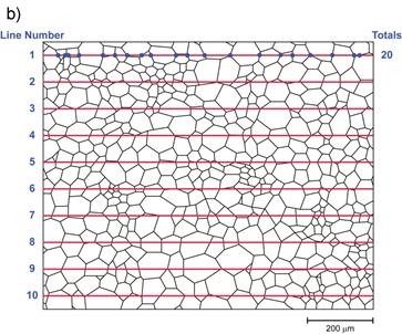
Figure 2 – The linear intercept method for grain size determination

The analysis proceeds as follows, using the procedures shown in Figure 2 and Table 1.

1) Draw a series of lines on the image. These lines can be spaced equally, but should be randomly placed and should be spaced sufficiently that no grain is crossed by two or more lines, in order to respect the random sampling criterion for us to be able to statistically analyse our results. See Figure 2a.

2) For the first line, identify the number of times that line crosses a grain boundary and count the total. This is shown in Figure 2b

3) Repeat for all of the lines (Figure 2c). The measurement is performed on a line by line basis as this allows each line to be treated as a measurement of the grain size. The results could be put together and treated as one sample, but in this case we would not be able to use the statistical analysis given here, and would have to estimate the error using the equations discussed later in this lecture. Either method is equally valid.

4) Measure the real length of the lines used (using the scale bar or magnification of the image). In the case of this example it is 1mm.

5) For each line, i, divide this total length by the number of grain boundaries to get the linear intercept length (Table 1, column 3).

6) These linear intercept lengths are summed, and divided by the total number of lines to get the mean linear intercept length (Table 1, column 3).

7) The difference of the linear intercept length of each line L _i from the mean linear intercept length is calculated and squared (Table 1, column 4).

8) This data is then used to calculate the standard deviation of the measurements using the equation given in the lecture on statistics (Table 1, column 4).

9) From the standard deviation, the standard error can be calculated using:

where n is our number of lines.

10) From the standard error, the 95% confidence limit can be calculated using the relevant t-value (e.g. from the table given in the lecture on Statistics and the result of the measurement expressed according to:

Line Number, i	No. of Grain Boundaries, NL	Linear Intercept Length, L i (µm)	Difference from sample mean
		50.0	38.1
		38.5	28.7
		40.0	14.6
		47.6	14.4
		40.0	14.6
		40.0	14.6
		38.5	28.8
		52.6	77.5
		47.6	14.4
		43.5	0.12
		ΣL i = 438.3	= 27.33
		ΣL i / 10 = 43.8 µm	s = 5.2

Table 1 – The calculation of grain size using the linear intercept method

In the case of this example, we can therefore express the mean grain size of the microstructure in Figure 1 with 95% confidence limits as being 43.8 ± 3.7 µm (given that S(L)=1.65 and t_{(95, n -1)} for n =10 is 2.262). Unlike when we were measuring the volume fraction, our parameter now has units, and it is important that these be given. Looking at Figure 1 the grain size found seems reasonable, but it is important to note that the range of confidence in our measurement does not relate to the range of grain sizes present in the material; in fact, the method of linear intercepts cannot capture information about the range of grain sizes present.

Дата добавления: 2015-10-26