B) Local trend approximation 1 страница

valueseries

past future

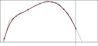
Fig. 3.1. Schematic representation of (a) a local level model; and (b) a local trendmodel.

40 3 Linear Innovations State Space Models

The final local level is projected into the future to give predictions. As the approximation is only effective in a small neighborhood, predictions generated this way are only likely to be reliable in the shorter term.

The second special case involves a first-order polynomial approximation. At each point, the data path is approximated by a straight line. In the deter-ministic world of analysis, this line would be tangential to the data path at the selected point. In the stochastic world of time series data, it can only be said that the line has a similar height and a similar slope to the data path. Randomness means that the line is not exactly tangential. The approximat-ing line changes over time, as depicted in Fig. 3.1b, to reflect the changing shape of the data path. The state of the process is now summarized by the level and the slope at each point of the path. The stochastic representation is based on the assumption that the gaps between successive slopes are Gaus-sian random variables with a zero mean. Note that the prediction is obtained by projecting the last linear approximation into the future.

It is possible to move beyond linear functions to higher order polynomials with quadratic or cubic terms. However, these extensions are rarely used in practice. It is commonly thought that the randomness found in real time series typically swamps and hides the effects of curvature.

Another strategy that does often bear fruit is the search for periodic behavior in time series caused by seasonal effects. Ignoring growth for the moment, the level in a particular month may be closer to the level in the corresponding month in the previous year than to the level in the preceding month. This leads to seasonal state space models.

3.4.1 Local Level Model: ETS(A,N,N)

The simplest way to transmit the history of a process is through a single state, __t, called the level. The resulting state space model is defined by the equations

yt = _t− 1	+ ε t,	(3.10a)
_t = _t− 1	+ αε t,	(3.10b)

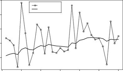
where ε _t ∼ NID(0, σ ²). It conforms to a state space structure with x_t = __t, w =1, F =1 and g = α. The values that are generated by this stochasticmodel are randomly scattered about the (local) levels as described in (3.10a). This is illustrated in Fig. 3.2 with a simulated series.

In demand applications, the level __{t− 1} represents the anticipated demand for period t, and ε _t represents the unanticipated demand. Changes to the underlying level may be induced by changes in the customer base such as the arrival of new customers, or by new competitors entering the market. Changes like these transcend a single period and must affect the underlying level. It is assumed that the unanticipated demand includes a persistent and

				3.4	Basic Special Cases
		Observed data
		Level
y

Time period

Fig. 3.2. Simulated series from the ETS(A,N,N) model. Here α =0.1 and σ =5.

a temporary effect; αε _t denotes the persistent effect, feeding through to future periods via the (local) levels governed by (3.10b).

The degree of change of successive levels is governed by the size of the smoothing parameter α. The cases where α = 0 and α = 1 are of special interest.

Case: α = 0 The local levels do not change at all when α = 0. Their com-mon level is then referred to as the global level. Successive values of the series y_t are independently and identically distributed. Its moments do not change over time.

Case: α = 1 The model reverts to a random walk y_t = y_{t− 1} + ε _t. Successive values of the time series y_t are clearly dependent.

The special case of transformation (3.3) for model (3.10) is

^{y ˆ} t|t− 1= ^_t− 1^,

ε t = yt − _t− 1, _t = _t− 1+ αε t.

It corresponds to simple exponential smoothing (Brown 1959), one of the most widely used methods of forecasting in business applications. It is a simple recursive scheme for calculating the innovations from the raw data. Equation (3.4) reduces to

_t = (1 −α) _t− 1 + αyt.

(3.11)

42 3 Linear Innovations State Space Models

The one-step-ahead predictions obtained from this scheme are linearly dependent on earlier series values. Equation (3.6) indicates that

t− 1
y ˆ t +1 |t = (1 − α) ^t _ 0+ α ∑(1 − α) ^j yt−j.	(3.12)

j =0

This is a linear function of the data and seed level. Ignoring the first term (which is negligible for large values of t and | 1 − α| < 1), the prediction y ˆ _{t|t− 1}is an exponentially weighted average of past observations. The coefficientsdepend on the “discount factor” 1 − α. If | 1 − α| < 1, then the coefficients become smaller as j increases. That is, the stability condition is satisfied if and only if 0 < α < 2. The coefficients are positive if and only if 0 < (1 − α) < 1, and (3.11) can then be interpreted as a weighted average of the past level __{t− 1} and the current series value y_t. Thus, the prediction can only be interpreted as a weighted average if 0 < α < 1.

Consequently, there are two possible ranges for α that have been pro-posed: 0 < α < 2 on the basis of a stability argument, and 0 < α < 1 on the basis of an interpretation as a weighted average. The narrower range is widely used in practice.

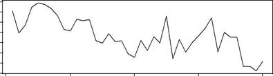
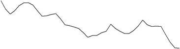
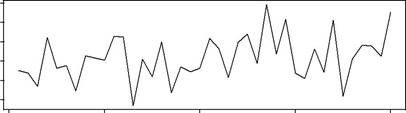
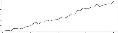
The impact of various values of α may be discerned from Fig. 3.3. It shows simulated time series from an ETS(A,N,N) model with _ ₀ = 100 and σ = 5 for various values of α. The same random number stream from a Gaussian distribution was used for the three series, so that any perceived differences can be attributed entirely to changes in α. For the case α = 0.1, the underlying level is reasonably stable. The plot has a jagged appearance because there is a tendency for the series to switch direction between successive observations. This is a consequence of the fact, shown in Chap. 11, that successive first-differences of the series, ∆ y_t and ∆ y_{t− 1}, are negatively correlated when α is restricted to the interval (0, 1). When α = 0.5, the underlying level displays a much greater tendency to change. There is still a tendency for successive observations to move in opposite directions. In the case α = 1.5, there is an even greater tendency for the underlying level to change. However, the series is much smoother. This reflects the fact, also established in Chap. 11, that successive first-differences of the series are positively correlated for cases where α lies in the interval (1, 2).

3.4.2 Local Trend Model: ETS(A,A,N)

The local level model can be augmented by a growth rate b_t to give

yt = _t− 1+ bt− 1	+ ε t,	(3.13a)
_t = _t− 1+ bt− 1	+ αε t,	(3.13b)
bt = bt− 1+ βε t,		(3.13c)

3.4 Basic Special Cases

			α = 0.1
y

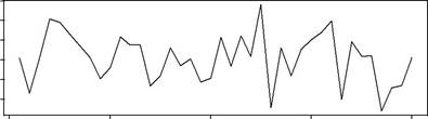
Time period

		α = 0.5
y
−40

Time period

		α = 1.5
−50
y
−150
−250

Time period

Fig. 3.3. Comparison of simulated time series from a local level model. Here σ =5.

where there are now two smoothing parameters α and β. The growth rate (or slope) b_t may be positive, zero or negative. Model (3.13) has a state space structure with

xt =^_ _t bt ^_ ^_,	w =^_	1 1	^_ _ ,	F =^_	1 1	_	and g = ^_ α β ^_ ^_.
0 1

The size of the smoothing parameters reflects the impact of the innova-tions on the level and growth rate. Figure 3.4 shows simulated values from the model for different settings of the smoothing parameters. When β = 0, the growth rate is constant over time. If, in addition, α = 0, the level changes at a constant rate over time. That is, there is no random change in the level or growth. This case will be called a global trend. The constant growth rate is sometimes interpreted as a long-term growth rate. For other values of the smoothing parameters, the growth rate follows a random walk over time. As

44 3 Linear Innovations State Space Models

		α = 0 and β = 0
y
		Time period

		α = 0.5 and β = 0.1
y
		Time period

		α = 1.2 and β = 1
y
		Time period

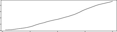
Fig. 3.4. Comparison of simulated time series from a local trend model. Here σ =5.

the smoothing parameters increase in size, there is a tendency for the series to become smoother.

For this model, the transformation (3.3) of series values into innovations becomes

^{y ˆ} t|t− 1= ^_t− 1+ ^bt− 1^, ε t = yt − y ^ˆ t|t− 1,

_t = _t− 1+ bt− 1+ αε t, b_t = b_{t− 1}+ βε _t.

This corresponds to Holt’s linear exponential smoothing (Holt 1957). An equivalent system of equations is

^y ^ˆ t|t− 1= ^_t− 1+ ^bt− 1^,

(3.14a)

3.4 Basic Special Cases

ε t = yt − y ^ˆ t|t− 1,

__t = αy_t + (1 − α)(__{t − 1} + b_{t− 1}), b_t = β^∗ (__t − __{t− 1}) + (1 − β^∗) b_{t− 1},

(3.14b)

(3.14c)

(3.14d)

where β^∗ = β / α. The term __t − __{t− 1} is often interpreted as the “actual growth” as distinct from the predicted growth b_{t − 1}.

Equations (3.14c) and (3.14d) may be interpreted as weighted averages if 0 < α < 1 and 0 < β^∗ < 1, or equivalently, if 0 < α < 1 and 0 < β < α. These restrictions are commonly applied in practice. Alternatively, it can be shown (see Chap. 10) that the model is stable (i.e., the discount matrix D^j converges to 0 as j increases) when α > 0, β > 0 and 2 α + β < 4. This provides a much larger parameter region than is usually allowed.

3.4.3 Local Additive Seasonal Model: ETS(A,A,A)

For time series that exhibit seasonal patterns, the local trend model can be augmented by seasonal effects, denoted by s_t. Often the structure of the seasonal pattern changes over time in response to changes in tastes and tech-nology. For example, electricity demand used to peak in winter, but in some locations it now peaks in summer due to the growing prevalence of air con-ditioning. Thus, the formulae used to represent the seasonal effects should allow for the possibility of changing seasonal patterns. The ETS(A,A,A) model is

^yt = _t− 1+ bt− 1	+ st−m + ε t,	(3.15a)
_t = _t− 1+ bt− 1	+ αε t,	(3.15b)
bt = bt− 1+ βε t,		(3.15c)
st = st−m + γε t.		(3.15d)

This model corresponds to the first-order state space model where

		_t
		bt
		st
	^st− ..
xt =		,
.
s	t		m +1
	−

w =1 1 0 · · · 0 1,
		1 1 0 0			0 0				α
	0 1 0 0 ·^· ·^· ·^·	0 0
		β
		0 0 0 0	· · ·	0 1
F =	0 0 1 0	0 0	and g =		γ		.
		0 0 0 1	· · ·	0 0
		· · ·				.
		....	..				.
		.... ^..	.	..				.
		....	..
		0 0 0 0			1 0
			· · ·

+ (s_t−m + δ) + ε _t,

46 3 Linear Innovations State Space Models

Careful inspection of model (3.15) shows that the level and seasonal terms are confounded. If an arbitrary quantity δ is added to the seasonal elements and subtracted from the level, the following equations are obtained

yt = (_t− 1 − δ) + bt− 1

__t − δ = __{t− 1} − δ + b_{t− 1}+ αε _t,

b_t = b_{t− 1}+ βε _t,

(s_t + δ) = (s_t−m + δ) + γε _t,

which is equivalent to (3.15). To avoid this problem, it is desirable to con-strain the seasonal component so that any sequence {s_t, s_{t +1},..., s_{t + m− 1} } sums to zero (or at least has mean zero). The seasonal components are said to be normalized when this condition is true. Normalization of seasonal fac-tors involves a subtle modification of the model and will be addressed in Chap. 8. In the meantime, we can readily impose the constraint that the sea-sonal factors in the initial state x ₀ must sum to zero. This means that the seasonal components start off being normalized, although there is nothing to constrain them from drifting away from zero over time.

Дата добавления: 2015-10-24