Читайте также:
|
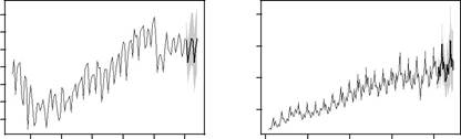
| Thousands of cars | 200 300 400 500 | Thousands of people | 200 400 600 800 | ||||
| Year |
| Year |
Fig. 2.1. Four time series showing pointobtained using exponential smoothing state
forecasts and 80% prediction intervals space models.
Cycle (C): A pattern that repeats with some regularity but with unknown and changing periodicity (e.g., a business cycle)
Irregular or error (E): The unpredictable component of the series
In this monograph, we focus primarily upon the three components T, S and E. Any cyclic element will be subsumed within the trend component unlessindicated otherwise.
These three components can be combined in a number of different ways. A purely additive model can be expressed as
y = T + S + E,
where the three components are added together to form the observed series. A purely multiplicative model is written as
y = T × S × E,
where the data are formed as the product of the three components. A sea-sonally adjusted series is then formed by extracting the seasonal component
| 2.2 Classification of Exponential Smoothing Methods |
from the data, leaving only the trend and error components. In the additive model, the seasonally adjusted series is y − S, while in the multiplica-tive model, the seasonally adjusted series is y / S. The reader should refer to Makridakis et al. (1998, Chap. 4) for a detailed discussion of seasonal adjustment and time series decomposition.
Other combinations, apart from simple addition and multiplication, are also possible. For example,
y = (T + S) × E
treats the irregular component as multiplicative but the other components as additive.1
2.2 Classification of Exponential Smoothing Methods
In exponential smoothing, we always start with the trend component, which is itself a combination of a level term (_) and a growth term (b). The level and growth can be combined in a number of ways, giving five future trend types. Let Th denote the forecast trend over the next h time periods, and let φ denote a damping parameter (0 < φ < 1). Then the five trend types orgrowth patterns are as follows:
| None: | Th | = _ |
| Additive: | Th | = _ + bh |
| Additive damped: | Th | = _ + (φ + φ 2 + · · · + φh) b |
| Multiplicative: | T | = _bh |
| h | ||
| Multiplicative damped: | Th = _b (φ + φ 2+ ··· + φh) |
A damped trend method is appropriate when there is a trend in the time series, but one believes that the growth rate at the end of the historical data is unlikely to continue more than a short time into the future. The equations for damped trend do what the name indicates: dampen the trend as the length of the forecast horizon increases. This often improves the forecast accuracy, particularly at long lead times.
Having chosen a trend component, we may introduce a seasonal compo-nent, either additively or multiplicatively. Finally, we include an error, either additively or multiplicatively. Historically, the nature of the error compo-nent has often been ignored, because the distinction between additive and multiplicative errors makes no difference to point forecasts.
If the error component is ignored, then we have the fifteen exponential smoothing methods given in the following table. This classification of meth-ods originated with Pegels’ (1969) taxonomy. This was later extended by

1 See Hyndman (2004) for further discussion of the possible combinations of these components.
| 2 Getting Started | ||||
| Trend component | Seasonal component | |||
| N | A | M | ||
| (None) | (Additive) | (Multiplicative) | ||
| N (None) | N,N | N,A | N,M | |
| A (Additive) | A,N | A,A | A,M | |
| Ad (Additive damped) | Ad,N | Ad,A | Ad,M | |
| M (Multiplicative) | M,N | M,A | M,M | |
| Md (Multiplicative damped) | Md,N | Md,A | Md,M |


Gardner (1985), modified by Hyndman et al. (2002), and extended again by Taylor (2003a), giving the fifteen methods in the above table.
Some of these methods are better known under other names. For exam-ple, cell (N,N) describes the simple exponential smoothing (or SES) method, cell (A,N) describes Holt’s linear method, and cell (Ad,N) describes the damped trend method. Holt-Winters’ additive method is given by cell (A,A), and Holt-Winters’ multiplicative method is given by cell (A,M). The other cells correspond to less commonly used but analogous methods.
For each of the 15 methods in the above table, there are two possible state space models, one corresponding to a model with additive errors and the other to a model with multiplicative errors. If the same parameter values are used, these two models give equivalent point forecasts although different prediction intervals. Thus, there are 30 potential models described in this classification.
We are careful to distinguish exponential smoothing methods from the underlying state space models. An exponential smoothing method is an algo-rithm for producing point forecasts only. The underlying stochastic state space model gives the same point forecasts, but also provides a framework for computing prediction intervals and other properties. The models are described in Sect. 2.5, but first we introduce the much older point-forecasting equations.
2.3 Point Forecasts for the Best-Known Methods
In this section, a simple introduction is provided to some of the best-known exponential smoothing methods—simple exponential smoothing (N,N), Holt’s linear method (A,N), the damped trend method (Ad,N) and Holt-Winters’ seasonal method (A,A and A,M). We denote the observed time series by y 1, y 2,..., yn. A forecast of yt + h based on all the data up to time t is denoted by y ˆ t + h|t. For one-step forecasts, we use the simpler notation y ˆ t +1 ≡ y ˆ t +1 |t. Usually, forecasts require some parameters to be estimated;but for the sake of simplicity it will be assumed for now that the values of all relevant parameters are known.
| 2.3 Point Forecasts for the Best-Known Methods |
2.3.1 Simple Exponential Smoothing (N,N Method)
Suppose we have observed data up to and including time t − 1, and we wish to forecast the next value of our time series, yt. Our forecast is denoted by y ˆ t. When the observation yt becomes available, the forecast error is found to be yt − y ˆ t. The method of simple exponential smoothing,2due to Brown’s workin the mid-1950s and published in Brown (1959), takes the forecast for the previous period and adjusts it using the forecast error. That is, the forecast for the next period is
| y ˆ t +1= y ˆ t + α (yt − y ˆ t), | (2.1) |
where α is a constant between 0 and 1.
It can be seen that the new forecast is simply the old forecast plus an adjustment for the error that occurred in the last forecast. When α has a value close to 1, the new forecast will include a substantial adjustment for the error in the previous forecast. Conversely, when α is close to 0, the new forecast will include very little adjustment.
Another way of writing (2.1) is
| y ˆ t +1= αyt + (1 − α) y ˆ t. | (2.2) |
The forecast y ˆ t +1 is based on weighting the most recent observation yt with a weight value α, and weighting the most recent forecast y ˆ t with a weight of 1 − α. Thus, it can be interpreted as a weighted average of the most recent forecast and the most recent observation.
The implications of exponential smoothing can be seen more easily if (2.2) is expanded by replacing y ˆ t with its components, as follows:
y ˆ t +1= αyt + (1 − α)[ αyt− 1+ (1 − α) y ˆ t− 1]= αyt + α (1 − α) yt− 1 + (1 − α)2 y ˆ t− 1.
If this substitution process is repeated by replacing y ˆ t− 1 with its components, y ˆ t − 2with its components, and so on, the result is
y ˆ t +1= αyt + α (1 − α) yt− 1+ α (1 − α)2 yt− 2+ α (1 − α)3 yt− 3
+ α (1 − α)4 yt− 4 + · · · + α (1 − α) t− 1 y 1 + (1 − α) t y ˆ1. (2.3)
So y ˆ t +1 represents a weighted moving average of all past observations with the weights decreasing exponentially; hence the name “exponential smooth-ing.” We note that the weight of y ˆ1 may be quite large when α is small and the time series is relatively short. The choice of starting value then becomes particularly important and is known as the “initialization problem,” which we discuss in detail in Sect. 2.6.
2 This method is also sometimes known as “ single exponential smoothing.”
14 2 Getting Started
For longer range forecasts, it is assumed that the forecast function is “flat.” That is,
| y ˆ | t + h|t | = y ˆ t +1, | h =2, 3,.... | |
A flat forecast function is used because simple exponential smoothing works best for data that have no trend, seasonality, or other underlying patterns.
Another way of writing this is to let _t = y ˆ t +1. Then y ˆ t + h|t = _t and _t = αyt + (1 − α) _t− 1. The value of _t is a measure of the “level” of the series at time t. While this may seem a cumbersome way to express the method, it provides a basis for generalizing exponential smoothing to allow for trend and seasonality.
In order to calculate the forecasts using SES, we need to specify the ini-tial value _ 0 = y ˆ1 and the parameter value α. Traditionally (particularly in the pre-computer age), y ˆ1 was set to be equal to the first observation and α was specified to be a small number, often 0.2. However, there are now much better ways of selecting these parameters, which we describe in Sect. 2.6.
2.3.2 Holt’s Linear Method (A,N Method)
Holt (1957)3 extended simple exponential smoothing to linear exponen-tial smoothing to allow forecasting of data with trends. The forecast for Holt’s linear exponential smoothing method is found using two smoothing constants, α and β∗ (with values between 0 and 1), and three equations:
| Level: | _t = αyt + (1 | − α)(_t− 1+ bt− 1), |
| Growth: | bt = β∗ (_t − _t− 1) + (1 − β∗) bt− 1, | |
| Forecast: | y ˆ t + h|t = _t + bt h. |
(2.4a)
(2.4b)
(2.4c)
Here _t denotes an estimate of the level of the series at time t and bt denotes an estimate of the slope (or growth) of the series at time t. Note that bt is a weighted average of the previous growth bt− 1 and an estimate of growth based on the difference between successive levels. The reason we use β∗ rather than β will become apparent when we introduce the state space models in Sect. 2.5.
In the special case where α = β∗, Holt’s method is equivalent to “Brown’s double exponential smoothing” (Brown 1959). Brown used a discounting argument to arrive at his forecasting equations, so 1 − α represents the common discount factor applied to both the level and trend components.
In Sect. 2.6 we describe how the procedure is initialized and how the parameters are estimated.
3 Reprinted as Holt (2004).
| 2.3 Point Forecasts for the Best-Known Methods |
One interesting special case of this method occurs when β∗ = 0. Then
Level: _t = αyt + (1 − α)(_t− 1 + b),
Forecast: y ˆ t + h|t = _t + bh.
This method is known as “SES with drift,” which is closely related to the “Theta method” of forecasting due to Assimakopoulos and Nikolopou-los (2000). The connection between these methods was demonstrated by Hyndman and Billah (2003).
2.3.3 Damped Trend Method (Ad,A Method)
Gardner and McKenzie (1985) proposed a modification of Holt’s linear method to allow the “damping” of trends. The equations for this method are:4
| Level: | _t = αyt + (1 − α)(_t− 1 + φbt− 1), | (2.5a) |
| Growth: | bt = β∗ (_t − _t− 1) + (1 − β∗) φbt− 1, | (2.5b) |
| Forecast: | y ˆ t + h|t = _t + (φ + φ 2+ · · · + φh) bt. | (2.5c) |
Thus, the growth for the one-step forecast of yt +1 is φbt, and the growth is dampened by a factor of φ for each additional future time period. If φ = 1, this method gives the same forecasts as Holt’s linear method. For 0 < φ < 1, as h → ∞ the forecasts approach an asymptote given by _t + φbt /(1 − φ). We usually restrict φ > 0 to avoid a negative coefficient being applied to bt− 1 in (2.5b), and φ ≤ 1 to avoid bt increasing exponentially.
2.3.4 Holt-Winters’ Trend and Seasonality Method
If the data have no trend or seasonal patterns, then simple exponential smoothing is appropriate. If the data exhibit a linear trend, then Holt’s linear method (or the damped method) is appropriate. But if the data are seasonal, these methods on their own cannot handle the problem well.
Holt (1957) proposed a method for seasonal data. His method was stud-ied by Winters (1960), and so now it is usually known as “Holt-Winters’ method” (see Sect. 1.3).
Holt-Winters’ method is based on three smoothing equations—one for the level, one for trend, and one for seasonality. It is similar to Holt’s lin-ear method, with one additional equation for dealing with seasonality. In fact, there are two different Holt-Winters’ methods, depending on whether seasonality is modeled in an additive or multiplicative way.
4 We use the same parameterization as Gardner and McKenzie (1985), which is slightly different from the parameterization proposed by Hyndman et al. (2002). This makes no difference to the value of the forecasts.
16 2 Getting Started
Multiplicative Seasonality (A,M Method)
The basic equations for Holt-Winters’ multiplicative method are as follows:
| yt | ||
| Level: | _t = α st−m + (1 − α)(_t− 1+ bt− 1) | (2.6a) |
| Growth: | bt = β∗ (_t − _t− 1) + (1 − β∗) bt− 1 | (2.6b) |
| Seasonal: | st = γyt /(_t− 1+ bt− 1) + (1 − γ) st−m | (2.6c) |
| Forecast: | y ˆ t + h|t = (_t + bt h) st−m + hm +, | (2.6d) |

where m is the length of seasonality (e.g., number of months or quarters in a year), _t represents the level of the series, bt denotes the growth, st is the seasonal component, y ˆ t + h|t is the forecast for h periods ahead, and h + m = [(h − 1)mod m ] +1. The parameters (α, β∗ and γ) are usually restrictedto lie between 0 and 1. The reader should refer to Sect. 2.6.2 for more details on restricting the values of the parameters. As with all exponential smooth-ing methods, we need initial values of the components and estimates of the parameter values. This is discussed in Sect. 2.6.
Equation (2.6c) is slightly different from the usual Holt-Winters’ equa-tions such as those in Makridakis et al. (1998) or Bowerman et al. (2005). These authors replace (2.6c) with
st = γyt / _t + (1 − γ) st−m.
The modification given in (2.6c) was proposed by Ord et al. (1997) to make the state space formulation simpler. It is equivalent to Archibald’s (1990) variation of Holt-Winters’ method. The modification makes a small but usually negligible difference to the forecasts.
Additive Seasonality (A,A Method)
The seasonal component in Holt-Winters’ method may also be treated addi-tively, although in practice this seems to be less commonly used. The basic equations for Holt-Winters’ additive method are as follows:
Level: _t = α (yt − st−m) + (1 − α)(_t− 1 + bt− 1)
Growth: bt = β∗ (_t − _t− 1) + (1 − β∗) bt− 1 Seasonal: st = γ (yt − _t− 1 − bt− 1) + (1 − γ) st−m Forecast: y ˆ t + h|t = _t + bt h + st−m + h + m.
(2.7a)
(2.7b)
(2.7c)
(2.7d)
The second of these equations is identical to (2.6b). The only differences in the other equations are that the seasonal indices are now added and subtracted instead of taking products and ratios.
| 2.5 State Space Models |
As with the multiplicative model, the usual equation given in textbooks for the seasonal term is slightly different from (2.7c). Most books use
st = γ∗ (yt − _t) + (1 − γ∗) st−m.
If _t is substituted using (2.7a), we obtain
st = γ∗ (1 − α)(yt − _t− 1 − bt− 1) + [1 − γ∗ (1 − α)] st−m.
Thus, we obtain identical forecasts using this approach by replacing γ in (2.7c) with γ∗ (1 − α).
2.4 Point Forecasts for All Methods
Table 2.1 gives recursive formulae for computing point forecasts h periods ahead for all of the exponential smoothing methods. In each case, _t denotes the series level at time t, bt denotes the slope at time t, st denotes the seasonal component of the series at time t, and m denotes the number of seasons in a year; α, β∗, γ and φ are constants, and φh = φ + φ 2 + · · · + φh.
Some interesting special cases can be obtained by setting the smoothing parameters to extreme values. For example, if α = 0, the level is constant over time; if β∗ = 0, the slope is constant over time; and if γ = 0, the sea-sonal pattern is constant over time. At the other extreme, na¨ıve forecasts (i.e., y ˆ t + h|t = yt for all h) are obtained using the (N,N) method with α = 1. Finally, the additive and multiplicative trend methods are special cases of their damped counterparts obtained by letting φ = 1.
2.5 State Space Models
We now introduce the state space models that underlie exponential smooth-ing methods. For each method, there are two models—a model with additive errors and a model with multiplicative errors. The point forecasts for the two models are identical (provided the same parameter values are used), but their prediction intervals will differ.
Дата добавления: 2015-10-24; просмотров: 168 | Нарушение авторских прав
| <== предыдущая страница | | | следующая страница ==> |
| Economic Applications: The Beveridge–Nelson | | | UK passenger motor vehicle production Overseas visitors to Australia 2 страница |