Laboratory work № 81

The elements of physical statistical distribution

THE AIM: determine what is statistical distribution is described thermoelectron gas and what is temperature of thermoelectron gas.

THE TASK: plot the graph of distribution of thermoelectrons over energies and compare it with Maxwell-Boltzmann’s function.

INSTRUMENTATION AND APPLIANCES: electron tube, milliampermeter, microampermeter, voltmeter, potentialmeter, variable resistor, power source.

Theory

1. Numerous events occur that cannot be predicted. These are called random events. The results obtained by observing numerous events of a single type, for example, analyzing the number of winning tickets for a large number of loan lotteries, may be summarized on the form of a so-called distribution curve. In the case of the analysis of the prize list, the distribution curve may be constructed on the basis of the date for the number of series of one hundred bonds for which there was one winner, two winner, etc.

If we construct a graph, plotting the random quantity along the horizontal axis and the number of random events along the vertical axis, the obtained curve is a distribution curve. An example of such a curve is shown in Figure 4.1. The curve is drawn through the mid-points of the tops of the rectangles. Each rectangle has an area equal to the number of times a random event occurred for the quantity lying in the given interval.

We call the distribution law of one or another quantity a statistical law. It is more accurately given the greater the number of events used to determine each ordinate of the curve.

Naturally, knowing the distribution curve does not enable us to predict the number of a bond that will win in the lottery. However, we can say, for example, what portion of the series consisting of one hundred numbers each will have one winner. The greater the number of bonds used in the analysis, the greater the accuracy of this prediction.

Figure 4.1

Certain ideas about the distribution of particles follow immediately from the chaotic nature of thermal motion.

Let us consider a small volume of space – a cube at point x, y, z whose sides are ∆ x, ∆ y, ∆ z.

Assume a considerable number of particles to be contained in this cube. We shall consider these particles having velocity components in the ranges from v _x to v _x + ∆ v _x, v_y to v _y + ∆ v _y and v _z to v _z + ∆ v _z. The magnitudes of ∆ v _x, ∆ v _y and ∆ v _z are such that a large number of particles are contained in the indicated interval of velocities. The kinetic energy of a particle is determined by the value of the velocity and the potential energy of a particle in an external field depends on the coordinates of the particle in space, all the particles segregated by us have, practically, one and the same energy e.

Boltzmann's law gives a general expression for the number of particles whose coordinates are in the neighborhood of x, y, z and velocities in the neighborhood of v_x, v_y, v_z. This number is

, (4.1)

where A is a constant, T is the absolute temperature and k is Boltzmann's constant.

The energy in to exponent is equal

. (4.2)

Hence

. (4.3)

Boltzmann's law or Boltzmann's distribution shows that the largest energy corresponds to the lowest number of particles whose velocities and coordinates lie in the given interval.

The velocity distribution of molecules, first determinated theoretically by Maxwell, may be considered to be a consequence of Boltzmann's law. We are interested in the number of molecules having a speed from v to v + ∆ v, where

. (4.4)

The number of molecules is the same for all cubes of volume ∆ v _x, ∆ v _y, ∆ v _z located within a spherical shell of radius v to v + ∆ v. The number of molecules having velocities in the range from v to v + ∆ v is proportional to the volume of the spherical shell, i.e. 4 πv ²∆ v. Thus, if the number of molecules contained in one cube is equal to

. (4.5)

The number of molecules contained in the spherical shell is represented by the formula:

. (4.6)

If n is the all number of molecules, then

, (4.7)

where f (v) is the function of velocity distribution.

The number of particles having energy in the ranges from ε to ε + dε is:

. (4.8)

From this formula following that the function of energy distribution is

. (4.9)

An example of such function of energy distribution is shown in Figure 4.2.

Figure 4.2

The square between the curve f (ε) and the horizontal axis ε is equal unit. For it following that

. (4.10)

This formula is normalization function of energy distribution. By normalization constant A may be written in the form

. (4.11)

2. Electrons at lower level practically do not take part in interactions between atoms. We must to understand the behavior of upper band electrons. Since we are dealing with a very large number of electrons, it is natural to use statistical physics methods and consider an aggregate of such electrons as a kind of gas.

The state of each electron of such a gas may be represented by a point (p _x, p _y, p _z) in momentum space. The energy of an electron depends on its momentum. Let us assume that the electrons behave like free particles.

If the electrons are free, the relationship between their energy and momentum is given by the formula

, (4.12)

where p is determined by

. (4.13)

This means that in momentum space a surface of equal energy is a sphere. It is customary to call such a sphere a Fermi sphere. We can say, that the states of an electron gas are contained in a sphere of radius

(4.14)

According to the principle of uncertainly, the projection of the momentum of a particle in a metal body of linear dimension L cannot determinates with greater accuracy than h/L, where h is Plank's constant. Therefore, in momentum space, the concept of a point should be replaced by the concept of a cell of volume h³/V, where V is the volume of the metal body under consideration. One of the basic postulates of the theory is that such as cell represents a quantum start and that it can contain no more than two electrons of opposite spins.

If there electrons in a volume V in the under consideration, then N /2 cells are occupied, i.e., the volume

. (4.15)

This is the volume of a Fermi sphere of radius p _max.

Thus,

. (4.16)

The above discussion assumed that the temperature is at absolute zero. At a higher temperature, electrons may pass over into momentum-space cells which correspond to higher energy.

The distribution of electrons according to energy at a given temperature may be calculated.

On the basic of the Pauli exclusion principle, we can construct a Fermi-Dirac statistics, in which the function is replaced by the expression:

. (4.17)

where ε _max is the maximum possible energy of the electrons at absolute zero. Figure 4.3 shows the dependence of the Fermi-Dirac function on ε when T >0 K

3. The escape of electrons from a metal upon heating is known as thermoionic emission. When the temperature is raised, electrons are excited, some of them acquiring a sufficient velocity in the direction perpendicular to the surface of the material to surmount the potential barrier ε.

Figure 4.3

An electron gas obeys Fermi-Dirac statistics, according to which the number of electrons having an energy ε is proportional to the expression

. (4.18)

But we are interested in the energies, which considerably greater than the zero-level energy μ. At absolute zero, electrons have a limiting energy μ. In the model of an electron gas, μ corresponds to a Fermi surface. Therefore it is accurate enough to reduce the above expression to

, (4.19)

where ф – work function is stopping potential. Thus, we may determine the number of electrons having energy equal to the height of the potential well. It may be rigorously proved that the thermionic emission current is proportional to this expression.

The circuit shown is Figure 4.4 may be used to measure the thermionic current.

Figure 4.4

The diode D which is shown diagrammatically consist of a filament F and a metallic plate P, both seated in a vacuum tube. The filament is heated by electric current from a battery A. Another battery B and galvanometer G are connected in series between the plate and one side of the filament. When the positive terminal of B is connected no current flows through the circuit; the galvanometer which registers the current reads zero.

The explanation of this behavior is that the filament when heated gives off negative electrons; hence, each time the plate is positive in relation to the filament, the electrons become attracted to the plate and flow through the circuit to the filament. When, however, the plate is negative in relation to the filament, the plate repels the electrons with the result that no current flow in the circuit.

If the filament is heated to a given temperature T, some of the free electrons of the metal evaporate from the filament into the space surrounding it. These from an electron gas around the filament. A state of equilibrium results when as many electrons leave the filament as re-enter it from the electron gas around it.

When a difference of potential exist between the filament and the plate, so that "+" on the plate and "-" on the filament, we have accelerating potential and electrons are attracted to the plate and other electrons evaporate from the filament to replace them. If a difference of potential between the filament and the plate so that “-“on the plate “+” on the filament then we have counter potential and electrons are repulsed from plate.

The number of electrons which create electronic current between the filament and the plate given the following expression:

, (4.20)

where B is coefficient; A _e is work function.

Then a current is measured by galvanometer G is determined by formula

, (4.21)

where C is new coefficient.

If on the plate negative potential exist relatively of the filament (counter potential) then it is equivalent of a rise of the work function. In this case for plates current we have

. (4.22)

After to take a logarithm

, (4.23)

or

. (4.24)

Those formulas give us a possible to determine the absolute temperature T of the filament if we draw the graph of ln I against U _count, how it shown from Figure 4.5.

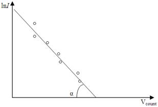
Figure 4.5

Дата добавления: 2015-10-29